I will argue that it is a category mistake to regard mathematics as “physically real”. I will quote D. E. Littlewood from his remarkable book “The Skeleton Key of Mathematics”:
“A trained sheepdog may perceive the significance of two, three or five sheep, and may know that two sheep and three sheep make five sheep. But very likely the knowledge would tell him nothing concerning, say horses. A child learns that two fingers and three fingers make five fingers, that two beads and three beads make five beads. The irrelevance of the fingers or the beads or the exact nature of the things that are counted becomes evident, and by the process of abstraction the universal truth that 2+3=5 becomes evident.”
I can just hear someone pouncing on Littlewood’s phrase “universal truth”, but that is not the reason I quote this paragraph. I quote it to remind that the essence of mathematics is never in the particular way it is represented, but in the concept that it brings forth, and the unification of particulars that it embodies.
One might hypothesize that any mathematical system will find natural realizations. This is not the same as saying that the mathematics itself is realized. The point of an abstraction is that it is not, as an abstraction, realized. The set { { }, { { } } } has 2 elements, but it is not the number 2. The number 2 is nowhere “in the world”.
I argue that one should understand from the outset that mathematics is distinct from the physical. Then it is possible to get on with the remarkable task of finding how mathematics fits with the physical, from the fact that we can represent numbers by rows of marks | , ||, |||, ||||, |||||, ||||||, …
(and note that whenever you do something concrete like this it only works for a while and then gets away from the abstraction living on as clear as ever, while the marks get hard to organize and count) to the intricate relationships of the representations of the symmetric groups with particle physics (bringing us back ’round to Littlewood and the Littlewood Richardson rule that appears to be the right abstraction behind elementary particle interactions).
Search for the right conceptual match between mathematics and phenomena, physical and computational. Understand that mathematics is distinct from its instances. And yet our understanding of the abstractions is utterly dependent on knowing more and more about their instantiations. The domains of the physical and the conceptual are distinct and they are mutually supporting.
It is very hard to take this point of view because we do not usually look carefully enough at our mathematics to distinguish the abstract part from the concrete or formal part. The key is in the seeing of the pattern, not in the mechanical work of the computation. The work of the computation occurs in physicality. The seeing of the pattern, the understanding of its generality occurs in the conceptual domain.
Conceptual and physical domains are interlocked in our understanding.

 where
where 


![\displaystyle [a,b] + [c,d]\eta = \left(\begin{array}{cc} a&c\\ d&b \end{array}\right).](https://s0.wp.com/latex.php?latex=%5Cdisplaystyle+%5Ba%2Cb%5D+%2B+%5Bc%2Cd%5D%5Ceta+%3D+%5Cleft%28%5Cbegin%7Barray%7D%7Bcc%7D+a%26c%5C%5C+d%26b+%5Cend%7Barray%7D%5Cright%29.&bg=ffffff&fg=000000&s=0&c=20201002)
![\displaystyle [x,y] = \left(\begin{array}{cc} x&0\\ 0&y \end{array}\right).](https://s0.wp.com/latex.php?latex=%5Cdisplaystyle+%5Bx%2Cy%5D+%3D+%5Cleft%28%5Cbegin%7Barray%7D%7Bcc%7D+x%260%5C%5C+0%26y+%5Cend%7Barray%7D%5Cright%29.&bg=ffffff&fg=000000&s=0&c=20201002)
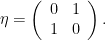
![\displaystyle ([a,b] + [c,d]\eta)([e,f]+[g,h]\eta) =](https://s0.wp.com/latex.php?latex=%5Cdisplaystyle+%28%5Ba%2Cb%5D+%2B+%5Bc%2Cd%5D%5Ceta%29%28%5Be%2Cf%5D%2B%5Bg%2Ch%5D%5Ceta%29+%3D+&bg=ffffff&fg=000000&s=0&c=20201002)
![\displaystyle [a,b][e,f] + [c,d]\eta[g,h]\eta + [a,b][g,h]\eta + [c,d]\eta[e,f] =](https://s0.wp.com/latex.php?latex=%5Cdisplaystyle+%5Ba%2Cb%5D%5Be%2Cf%5D+%2B+%5Bc%2Cd%5D%5Ceta%5Bg%2Ch%5D%5Ceta+%2B+%5Ba%2Cb%5D%5Bg%2Ch%5D%5Ceta+%2B+%5Bc%2Cd%5D%5Ceta%5Be%2Cf%5D+%3D&bg=ffffff&fg=000000&s=0&c=20201002)
![\displaystyle [ae,bf] + [c,d][h,g] +( [ag, bh] + [c,d][f,e])\eta =](https://s0.wp.com/latex.php?latex=%5Cdisplaystyle+%5Bae%2Cbf%5D+%2B+%5Bc%2Cd%5D%5Bh%2Cg%5D+%2B%28+%5Bag%2C+bh%5D+%2B+%5Bc%2Cd%5D%5Bf%2Ce%5D%29%5Ceta+%3D+&bg=ffffff&fg=000000&s=0&c=20201002)
![\displaystyle [ae,bf] +[ch,dg] + ( [ag, bh] + [cf,de])\eta =](https://s0.wp.com/latex.php?latex=%5Cdisplaystyle+%5Bae%2Cbf%5D+%2B%5Bch%2Cdg%5D+%2B+%28+%5Bag%2C+bh%5D+%2B+%5Bcf%2Cde%5D%29%5Ceta+%3D+&bg=ffffff&fg=000000&s=0&c=20201002)
![\displaystyle [ae+ch, dg+bf] + [ag + cf, de+bh]\eta.](https://s0.wp.com/latex.php?latex=%5Cdisplaystyle+%5Bae%2Bch%2C+dg%2Bbf%5D+%2B+%5Bag+%2B+cf%2C+de%2Bbh%5D%5Ceta.&bg=ffffff&fg=000000&s=0&c=20201002)
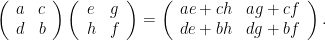
![{[a,d]}](https://s0.wp.com/latex.php?latex=%7B%5Ba%2Cd%5D%7D&bg=ffffff&fg=000000&s=0&c=20201002) and
and ![{[b,c]}](https://s0.wp.com/latex.php?latex=%7B%5Bb%2Cc%5D%7D&bg=ffffff&fg=000000&s=0&c=20201002) via the shift operation
via the shift operation ![{\eta [x,y] = [y,x] \eta}](https://s0.wp.com/latex.php?latex=%7B%5Ceta+%5Bx%2Cy%5D+%3D+%5By%2Cx%5D+%5Ceta%7D&bg=ffffff&fg=000000&s=0&c=20201002) which we shall denote by an overbar as shown below
which we shall denote by an overbar as shown below![\displaystyle \overline{[x,y]} = [y,x].](https://s0.wp.com/latex.php?latex=%5Cdisplaystyle+%5Coverline%7B%5Bx%2Cy%5D%7D+%3D+%5By%2Cx%5D.&bg=ffffff&fg=000000&s=0&c=20201002)
![{A = [a,d]}](https://s0.wp.com/latex.php?latex=%7BA+%3D+%5Ba%2Cd%5D%7D&bg=ffffff&fg=000000&s=0&c=20201002) and
and ![{B=[b,c]}](https://s0.wp.com/latex.php?latex=%7BB%3D%5Bb%2Cc%5D%7D&bg=ffffff&fg=000000&s=0&c=20201002) , we see that the four matrices seen in the grid are
, we see that the four matrices seen in the grid are
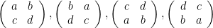
 has the effect of rotating an iterant by ninety degrees in the formal plane. Ordinary matrix multiplication can be written in a concise form using the following rules:

![\displaystyle \left(\begin{array}{cc} a&b\\ c&d \end{array}\right) = \left(\begin{array}{cc} a&0\\ 0&d \end{array}\right) \left(\begin{array}{cc} 1&0\\ 0&1 \end{array}\right) + \left(\begin{array}{cc} b&0\\ 0&c \end{array}\right) \left(\begin{array}{cc} 0&1\\ 1&0 \end{array}\right) = [a,d]1 + [b,c]\eta.](https://s0.wp.com/latex.php?latex=%5Cdisplaystyle+%5Cleft%28%5Cbegin%7Barray%7D%7Bcc%7D+a%26b%5C%5C+c%26d+%5Cend%7Barray%7D%5Cright%29+%3D+%5Cleft%28%5Cbegin%7Barray%7D%7Bcc%7D+a%260%5C%5C+0%26d+%5Cend%7Barray%7D%5Cright%29+%5Cleft%28%5Cbegin%7Barray%7D%7Bcc%7D+1%260%5C%5C+0%261+%5Cend%7Barray%7D%5Cright%29+%2B+%5Cleft%28%5Cbegin%7Barray%7D%7Bcc%7D+b%260%5C%5C+0%26c+%5Cend%7Barray%7D%5Cright%29+%5Cleft%28%5Cbegin%7Barray%7D%7Bcc%7D+0%261%5C%5C+1%260+%5Cend%7Barray%7D%5Cright%29+%3D+%5Ba%2Cd%5D1+%2B+%5Bb%2Cc%5D%5Ceta.&bg=ffffff&fg=000000&s=0&c=20201002)
![\displaystyle [a,d] = \left(\begin{array}{cc} a&0\\ 0&d \end{array}\right),](https://s0.wp.com/latex.php?latex=%5Cdisplaystyle+%5Ba%2Cd%5D+%3D+%5Cleft%28%5Cbegin%7Barray%7D%7Bcc%7D+a%260%5C%5C+0%26d+%5Cend%7Barray%7D%5Cright%29%2C&bg=ffffff&fg=000000&s=0&c=20201002)

![{[b,c]\eta}](https://s0.wp.com/latex.php?latex=%7B%5Bb%2Cc%5D%5Ceta%7D&bg=ffffff&fg=000000&s=0&c=20201002) corresponds to the product of a diagonal matrix and the permutation matrix.
corresponds to the product of a diagonal matrix and the permutation matrix.![\displaystyle [b,c]\eta = \left(\begin{array}{cc} b&0\\ 0&c \end{array}\right) \left(\begin{array}{cc} 0&1\\ 1&0 \end{array}\right) = \left(\begin{array}{cc} 0&b\\ c&0 \end{array}\right).](https://s0.wp.com/latex.php?latex=%5Cdisplaystyle+%5Bb%2Cc%5D%5Ceta+%3D+%5Cleft%28%5Cbegin%7Barray%7D%7Bcc%7D+b%260%5C%5C+0%26c+%5Cend%7Barray%7D%5Cright%29+%5Cleft%28%5Cbegin%7Barray%7D%7Bcc%7D+0%261%5C%5C+1%260+%5Cend%7Barray%7D%5Cright%29+%3D+%5Cleft%28%5Cbegin%7Barray%7D%7Bcc%7D+0%26b%5C%5C+c%260+%5Cend%7Barray%7D%5Cright%29.&bg=ffffff&fg=000000&s=0&c=20201002)
![{ [a,d]1 + [b,c]\eta}](https://s0.wp.com/latex.php?latex=%7B+%5Ba%2Cd%5D1+%2B+%5Bb%2Cc%5D%5Ceta%7D&bg=ffffff&fg=000000&s=0&c=20201002) captures the whole of
captures the whole of  matrix algebra corresponds to the fact that a two by two matrix is combinatorially the union of the identity pattern (the diagonal) and the interchange pattern (the antidiagonal) that correspond to the operators
  and
and 

 and the anti-diagonal by
![\displaystyle \left(\begin{array}{cc} a&b\\ -b&a \end{array}\right) = [a,a] + [b,-b]\eta = a1 + b[1,-1]\eta = a + bi.](https://s0.wp.com/latex.php?latex=%5Cdisplaystyle+%5Cleft%28%5Cbegin%7Barray%7D%7Bcc%7D+a%26b%5C%5C+-b%26a+%5Cend%7Barray%7D%5Cright%29+%3D+%5Ba%2Ca%5D+%2B+%5Bb%2C-b%5D%5Ceta+%3D+a1+%2B+b%5B1%2C-1%5D%5Ceta+%3D+a+%2B+bi.&bg=ffffff&fg=000000&s=0&c=20201002)
 We will now see how to generalize this point of view to arbitrary finite groups.
![\displaystyle i = \epsilon \eta = [-1,1]\eta =\left(\begin{array}{cc} 0&1\\ -1&0 \end{array}\right).](https://s0.wp.com/latex.php?latex=%5Cdisplaystyle+i+%3D+%5Cepsilon+%5Ceta+%3D+%5B-1%2C1%5D%5Ceta+%3D%5Cleft%28%5Cbegin%7Barray%7D%7Bcc%7D+0%261%5C%5C+-1%260+%5Cend%7Barray%7D%5Cright%29.&bg=ffffff&fg=000000&s=0&c=20201002)


 by the formula
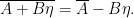

 while
while  so that
  . The basic operations in this algebra are those of epsilon and eta. Eta is the delay shift operator that reverses the components of the iterant. Epsilon negates one of the components, and leaves the order unchanged. The quaternions arise directly from these two operations once we construct an extra square root of minus one that commutes with them. Call this extra root of minus one
  . Then the quaternions are generated by


